Author: Star Li
This article is for industry learning and exchange only and does not constitute any investment reference. If you need to quote it, please indicate the source. For reprinting, please contact the IOSG team for authorization and reprinting instructions. Special thanks to author Star Li for providing the content!
Zero-knowledge proof (ZKP) technology is increasingly being used in privacy proofs, computation proofs, consensus proofs, and more. While looking for more and better applications, many people have gradually discovered that ZKP proof performance is a bottleneck. The Trapdoor Tech team has been deeply researching ZKP technology since 2019 and has been exploring efficient ZKP proof acceleration schemes. GPU or FPGA is currently a more common acceleration platform on the market. This article analyzes the advantages and disadvantages of accelerating ZKP proof calculation on FPGA and GPU, starting from the calculation of MSM.
TL; DR
- Three implications of blockchain technology for the beauty industry
- Discussion on the current technology stack controversy and trends of Bitcoin
- News Weekly | National standard “Reference Architecture for Blockchain and Distributed Ledger Technology” will be implemented on December 1st
ZKP is a technology with broad prospects for the future. More and more applications are beginning to adopt ZKP technology. However, there are many ZKP algorithms, and various projects use different ZKP algorithms. At the same time, the computational performance of ZKP proofs is relatively poor. This article analyzes the MSM algorithm, elliptic curve point addition algorithm, Montgomery multiplication algorithm, and more, and compares the performance differences between GPU and FPGA in BLS12_381 curve point addition. Overall, in terms of ZKP proof calculation, the short-term advantages of GPU are quite obvious, with high throughput, cost-effectiveness, programmability, and more. FPGA, on the other hand, has a certain advantage in power consumption. In the long run, it is possible to have FPGA chips suitable for ZKP calculation, or ASIC chips customized for ZKP.
ZKP Algorithm Complexity
ZKP is a general term for zero-knowledge proof technology. There are mainly two types of classification: zk-SNARK and zk-STARK. The commonly used algorithm for zk-SNARK is Groth16, PLONK, PLOOKUP, Marlin, and Halo/Halo2. The iteration of the zk-SNARK algorithm mainly follows two directions: 1/ whether a trusted setup is needed 2/ the performance of the circuit structure. The advantage of the zk-STARK algorithm is that no trusted setup is required, but the verification calculation amount is logarithmically linear.
Looking at the applications of zk-SNARK/zk-STARK algorithms, the zero-knowledge proof algorithms used by different projects are relatively scattered. In zk-SNARK algorithm applications, because the PLONK/Halo2 algorithm is universal (no trusted setup required), the application may become more and more widespread.
PLONK Proof Calculation Amount
Taking the PLONK algorithm as an example, let’s analyze the calculation amount of PLONK proofs.
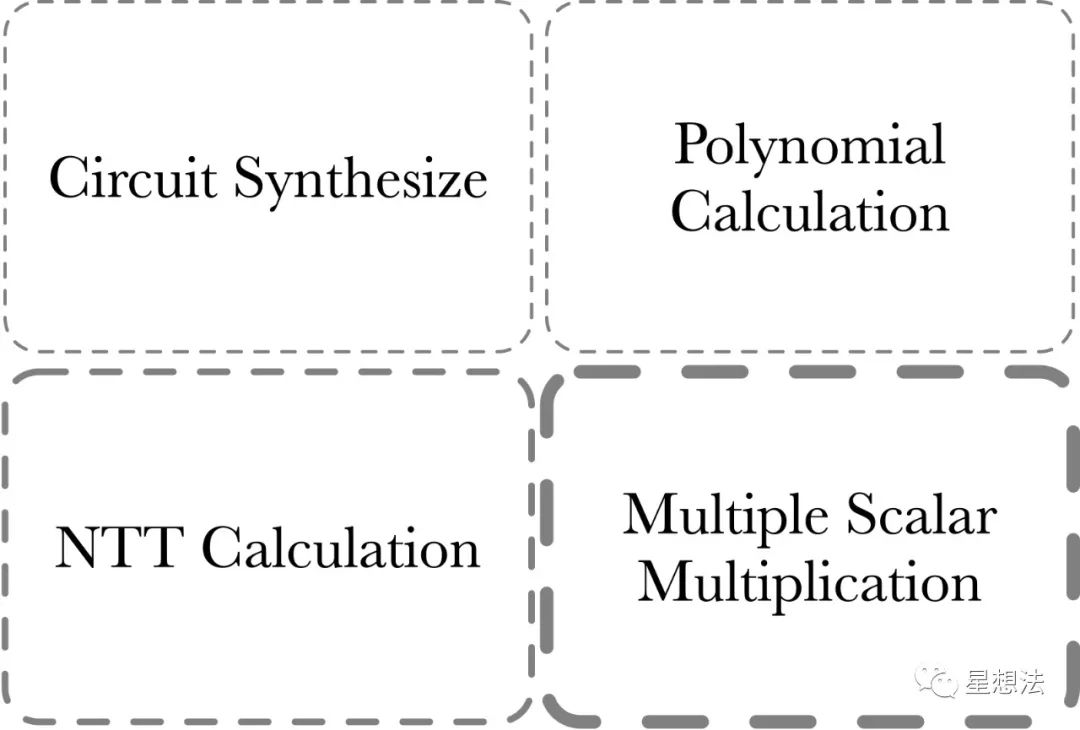
The calculation of the PLONK proof is composed of four parts:
1/ MSM – Multiple Scalar Multiplication. MSM is often used to calculate polynomial commitments.
2/ NTT Calculation – Transforming polynomials between point-value and coefficient representation.
3/ Polynomial Calculation – Polynomial addition, subtraction, multiplication, division, and evaluation.
4/ Circuit Synthesize – Circuit synthesis. This part of the calculation is related to the size/complexity of the circuit, and is more suitable for CPU calculation due to the large amount of judgment and loop logic and low parallelism. Generally speaking, the acceleration of zero-knowledge proof usually refers to the acceleration of the first three parts of the calculation. Among them, the calculation of MSM is relatively the largest, followed by NTT.
What’s MSM
MSM (Multiple Scalar Multiplication) refers to the calculation of the point corresponding to the sum of the results obtained by adding a series of points on an elliptic curve and their corresponding scalars.
For example, given a fixed set of points on an elliptic curve:
[G_1, G_2, G_3, …, G_n]
and randomly sampled scalars:
[s_1, s_2, s_3, …, s_n]
MSM is the calculation to get the Elliptic curve point Q:
Q = \sum_{i=1}^{n}s_i*G_i
The industry generally uses the Pippenger algorithm to optimize MSM calculation. Let’s take a closer look at the process of the Pippenger algorithm:
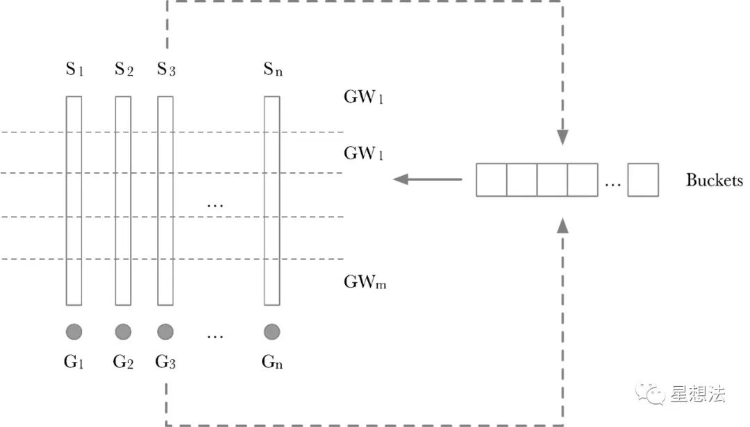
The calculation process of the Pippenger algorithm is divided into two steps:
1/ Scalar is split into windows. If the Scalar is 256 bits and one window is 8 bits, all Scalars are split into 256/8=32 windows. Each layer of windows uses a “Buckets” to temporarily store intermediate results. GW_x is the accumulated point on a layer. Calculating GW_x is also relatively simple, traverse each Scalar in a layer, and add the corresponding G_x to the corresponding position of the Buckets according to the value of Scalar on this layer as the Index. The principle is also relatively simple. If the coefficients added by two points are the same, add the two points first and then add one Scalar, instead of adding two Scalars to the two points and then accumulating.
2/ Each point calculated on the Window is accumulated through double-addition to obtain the final result. There are many variations of Pippenger’s algorithm. Regardless of the optimization algorithm used, the underlying calculation of the MSM algorithm is point addition on an elliptic curve. Different optimization algorithms correspond to different numbers of point additions.
Elliptic Curve Point Addition (Point Add)
You can view various algorithms for point addition on elliptic curves with “short Weierstrass” form on this website.
http://www.hyperelliptic.org/EFD/g1p/auto-shortw-jacobian-0.html#addition-madd-2007-bl
Assuming the Projective coordinates of the two points are (x1, y1, z1) and (x2, y2, z2), the result of point addition (x3, y3, z3) can be calculated through the following formula:
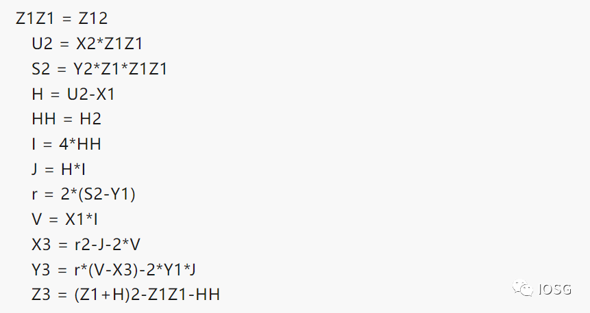
The reason for providing detailed calculation steps is to show that most of the calculation process is integer arithmetic. The bit width of the integers depends on the parameters of the elliptic curve. Here are some common bit widths of elliptic curves:
- BN256 – 256 bits
- BLS12_381 – 381 bits
- BLS12_377 – 377 bits
It is important to note that these integer operations are performed in a modular field. Modular addition/subtraction is relatively simple. The focus will be on the principles and implementation of modular multiplication.
Modular Multiplication
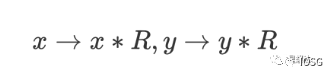
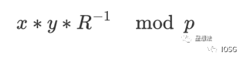
Given two values in a modular field: x and y. Modular multiplication computes x*y mod p. Note that the bit width of these integers is the bit width of the elliptic curve. The classical algorithm for modular multiplication is Montgomery Multiplication. Before performing Montgomery Multiplication, the multiplicand needs to be converted to the Montgomery representation:
The formula for Montgomery Multiplication is as follows:
There are many implementation algorithms for Montgomery Multiplication, such as CIOS (Coarsely Integrated Operand Scanning), FIOS (Finely Integrated Operand Scanning), and FIPS (Finely Integrated Product Scanning), etc. This article does not delve into the details of the implementation of various algorithms. Interested readers can study them on their own.
In order to compare the performance difference between FPGA and GPU, the most basic algorithm implementation method is chosen:
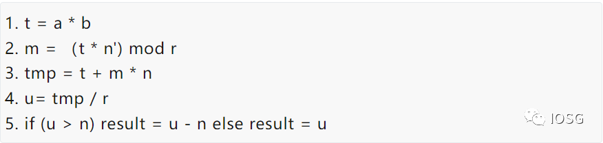
Simply put, the modular multiplication algorithm can be further divided into two types of calculations: large number multiplication and large number addition. After understanding the calculation logic of MSM, the performance (Throughput) of modular multiplication can be selected to compare the performance of FPGA and GPU.
Observation and Thinking
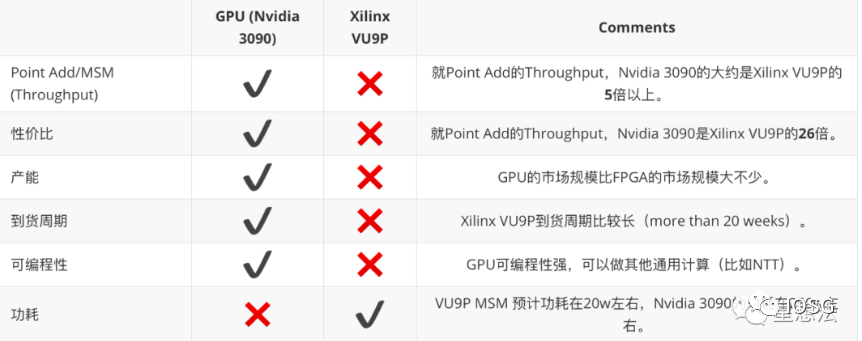
Under such an FPGA design, the throughput of the entire VU9P that can be provided for BLS12_381 elliptic curve point addition can be estimated. One point addition (add_mix method) requires about 12 modular multiplications. The system clock of FPGA is 450M.

Under the same modular multiplication/modular addition algorithm, using the same point addition algorithm, the point addition throughput of Nvidia 3090 (considering data transmission factors) exceeds 500M/s. Of course, the entire calculation involves multiple algorithms, and some algorithms may be suitable for FPGA, and some algorithms may be suitable for GPU. The reason for comparing the same algorithm is to compare the core computing capabilities of FPGA and GPU.
Based on the above results, summarizing the comparison of GPU and FPGA in ZKP proof performance:
Summary
More and more applications are beginning to use zero-knowledge proof technology. However, there are many ZKP algorithms, and various projects use different ZKP algorithms. From our practical engineering experience, FPGA is an option, but currently GPU is a cost-effective option. FPGA prefers deterministic calculation, and has the advantages of latency and power consumption. GPU has high programmability, relatively mature high-performance computing frameworks, short development iteration cycles, and prefers throughput scenarios.
Like what you're reading? Subscribe to our top stories.
We will continue to update Gambling Chain; if you have any questions or suggestions, please contact us!
